Blocks and Pipes¶

A block graph describes a logical computation encoded by surface code as a spacetime layout. Blocks represent operations on logical patches, and pipes connect their boundaries: temporal pipes continue a patch through time, while spatial pipes join patches for lattice surgery.

A block starts at an integer coordinate [x, y, z], with x and y describing space and z describing time. Its physical spacetime occupation can be larger or smaller than a \(1\times1\times1\) cell. For example, a taller cube spans several time cells, a Y block takes roughly half a cube’s duration, and a moving block extends across spatial cells. A pipe joins adjacent connectable positions on the blocks.

Supported blocks and pipes¶

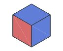
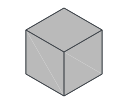
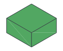
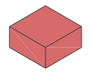
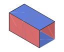
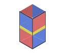
Let \(d\) be the code distance and \(s=2d+2\) the physical lattice pitch of one block cell. Space occupation counts physical-qubit lattice sites, including the boundary margin: a distance-\(d\) patch cell occupies \(s^2=(2d+2)^2\) sites. Time duration is the exact number of syndrome rounds. / denotes zero occupation or duration. Thumbnails show representative orientations.

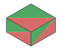
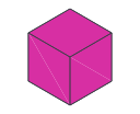
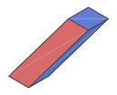
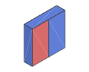
Circuit Constructions shows the physical realization of each family.

Special variants¶

Variable-height cubes. The default height=d gives \(d\) syndrome rounds. A height \(kd+n\) gives \(\lceil kd\rceil+n\) rounds and reserves \(\lceil k\rceil\) graph cells in time. The reserved spatial footprint remains \((2d+2)^2\).

At least two rounds are required. Spatially connected cubes share a height, and the next temporal block starts beyond the reserved cells.

Port roles. A Port has exactly one pipe and leaves the logical boundary open for an input, output, or module connection. Its role and pipe direction determine which interface it exposes.

Temporal Ports infer their role with role=auto; explicit temporal roles must agree with the pipe direction. Suitable input and output Ports can be filled with preparation and measurement boundaries for a closed experiment.

A multiplex Port combines an input and its continuing output at one spatial boundary. It follows the Z-port calling convention: Z-split the incoming qubit, connect one branch to the computation by a Z merge, and keep the other branch as the stationary output.[1] In Bloq, the virtual split exposes one temporal input and one retained output alongside the spatial connection. Their Z operators are correlated; their X operators belong to the full split relation. This lets arithmetic use the qubit’s Z value while retaining the qubit. Named readouts at a multiplex Port must be output-safe: Z support is allowed, while X or Y support on the retained output is rejected.

Y-basis initialization and measurement. A Y block with a +Z pipe initializes the future patch in \(+Y\); with a -Z pipe it measures the past patch in the Y basis.

Moving blocks. Walking (walk) and patch rotation (rotate) are the two moving block families. Walking moves one spatial cell by sliding along a spatial axis or gliding diagonally along both axes. Patch rotation turns the patch orientation by \(90^\circ\) and moves one cell along a spatial axis. Both advance one graph time layer and connect to temporal pipes at their start and end positions.

Compose blocks¶

Blocks acquire their logical meaning together with their pipe connections. For example, the following five-block layout gives the geometry of a logical S gate. The data patch runs from the input Port at [0, 0, 0] through an XZX cube to the output Port at [0, 0, 2]. An adjacent XZX cube initializes an ancilla in \(+X\). A spatial pipe joins it to the data patch, and a temporal pipe carries it to a Y-basis measurement.

Both examples place the blocks, connect them with pipes, and return the validated block graph.

import bloq


def build_graph():
    graph = bloq.BlockGraph()
    for position, kind in [
        ((0, 0, 0), "Port"),
        ((0, 0, 1), "XZX"),
        ((0, 0, 2), "Port"),
        ((1, 0, 1), "XZX"),
        ((1, 0, 2), "Y"),
    ]:
        graph.add_block(bloq.Block(position, kind))
    for position, direction in [
        ((0, 0, 0), "+Z"),
        ((0, 0, 1), "+Z"),
        ((0, 0, 1), "+X"),
        ((1, 0, 1), "+Z"),
    ]:
        graph.add_pipe(bloq.Pipe(position, direction))
    graph.validate()
    return graph

use bloq::prelude::*;

fn build_graph() -> Result<BlockGraph> {
    let mut graph = BlockGraph::new();
    for (position, kind) in [
        ([0, 0, 0], BlockKind::Port),
        ([0, 0, 1], BlockKind::Cube(CubeKind::XZX)),
        ([0, 0, 2], BlockKind::Port),
        ([1, 0, 1], BlockKind::Cube(CubeKind::XZX)),
        ([1, 0, 2], BlockKind::Y),
    ] {
        graph.try_add_block(Block::new(position, kind))?;
    }
    for (position, direction) in [
        ([0, 0, 0], Direction::ZPLUS),
        ([0, 0, 1], Direction::ZPLUS),
        ([0, 0, 1], Direction::XPLUS),
        ([1, 0, 1], Direction::ZPLUS),
    ] {
        graph.try_add_pipe(Pipe::new(position, direction))?;
    }
    graph.validate()?;
    Ok(graph)
}

Geometry exports¶

glTF exports logical blocks, pipes, colors, and supported surface overlays for visualization. The HTML viewer embeds the model and loads its renderer from a CDN, so displaying it requires network access. These files do not encode executable control dependencies or a physical quantum program. Exporting through the Rust graph API requires gltf; the CLI includes it.

Next, Actions introduces logical measurements and classical control to extend a block graph beyond its geometry.