Logical CNOT¶

This tutorial shows how to represent and compile a logical CNOT gate with Bloq, then simulate and decode it with Stim and PyMatching.

Install the tutorial’s sampling dependencies in your Python project:

uv add "bloq-py==0.1.1" stim pymatching

Build the block graph¶

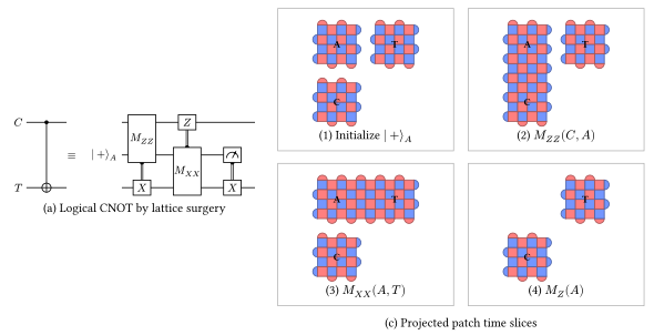
CNOT parity-measurement circuit with a plus-state ancilla, conditional X/Z corrections, and four lattice-surgery patch snapshots. — Logical CNOT via \(ZZ\) and \(XX\) parity measurements, ancilla \(Z\) readout, and measurement-dependent Pauli corrections.¶

graph = bloq.BlockGraph()
blocks = [
    ((0, 0, 0), "Port"), ((0, 0, 1), "ZXX"),
    ((0, 0, 2), "ZXZ"), ((0, 0, 3), "Port"),
    ((0, 1, 1), "ZXX"), ((0, 1, 2), "ZXZ"),
    ((1, 1, 0), "Port"), ((1, 1, 1), "ZXZ"),
    ((1, 1, 2), "ZXZ"), ((1, 1, 3), "Port"),
]
for position, kind in blocks:
    graph.add_block(bloq.Block(position, kind))
for position, direction in [
    ((0, 0, 0), "+Z"), ((0, 0, 1), "+Z"),
    ((0, 0, 1), "+Y"), ((0, 0, 2), "+Z"),
    ((0, 1, 1), "+Z"), ((0, 1, 2), "+X"),
    ((1, 1, 0), "+Z"), ((1, 1, 1), "+Z"),
    ((1, 1, 2), "+Z"),
]:
    graph.add_pipe(bloq.Pipe(position, direction))
graph.validate()
graph.save("cnot.blog")

Inspect the correlation surfaces¶

For control \(c\) and target \(t\), CNOT transports the Pauli operators as follows:

Input	Output
\(X_c\)	\(X_cX_t\)
\(Z_c\)	\(Z_c\)
\(X_t\)	\(X_t\)
\(Z_t\)	\(Z_cZ_t\)

Compute a generating basis and inspect its external support:

correlations = graph.stabilizers()
assert len(correlations) == 4
for row in correlations:
    print(row.kind, row.stabilizer.port_stabilizer)

Generators can be combined, so a returned row need not match one table row verbatim. The complete relation determines the map.

X control → X control · X target Z control → Z control X target → X target Z target → Z control · Z target

Read Correlation Surfaces for the signed algebra and decoder-corrected readout interpretation.

Compile and emit¶

program = bloq.compile(graph, distance=3)
program.validate()
program.save("cnot.bloqir")
Path("cnot.svg").write_text(program.to_svg(include_classical=True), encoding="utf-8")
circuit = bloq.emit_stim(program)
circuit.to_file("cnot.stim")

cnot.bloqir retains the physical program; cnot.svg shows its dependencies. cnot.stim is the static backend circuit. Its Ports are still ideal open boundaries: compilation has not chosen physical input states or measurements.

The CLI can perform the corresponding gallery workflow:

bloq compile --gallery cnot -d 3 --backend ir-text -o cnot.bloqir
bloq emit cnot.bloqir -o cnot.stim

Auto-fill a closed experiment¶

A block graph with open Ports represents a logical channel that can be simulated with ideal boundaries. To run a complete experiment on quantum hardware, prepare the input states and measure the outputs in chosen logical bases.

Automatic filling chooses compatible preparation/readout boundaries from the source correlation relation. It returns closed graphs and the relations each experiment measures. Select the first compatible variant here:

experiments = graph.fill_ports_auto()
closed, measured_relations = experiments[0]
assert closed.port_count == 0
closed.save("cnot.closed.blog")
closed_program = bloq.compile(closed, distance=3)
clean = bloq.emit_stim(closed_program)
detectors, observables = clean.compile_detector_sampler(seed=7).sample(
    shots=1024, separate_observables=True
)
assert not detectors.any()
assert not observables.any()

Sample and decode with noise¶

Apply a uniform depolarizing noise model with strength \(p=10^{-3}\), then sample detector events and decode with PyMatching:

import numpy as np
import pymatching

noisy = bloq.emit_stim(closed_program, noise=1e-3)
noisy.to_file("cnot.closed.stim")
model = noisy.detector_error_model(decompose_errors=True)
matching = pymatching.Matching.from_detector_error_model(model)
detectors, actual = noisy.compile_detector_sampler(seed=11).sample(
    shots=1024, separate_observables=True
)
predicted = matching.decode_batch(detectors)
failures = np.any(predicted != actual, axis=1)
print("noisy shots:", len(failures))
print("any-logical failures:", int(failures.sum()))

Download the complete runnable example. See Stim’s API reference for further sampling and detector-model options.

Simulation Results¶

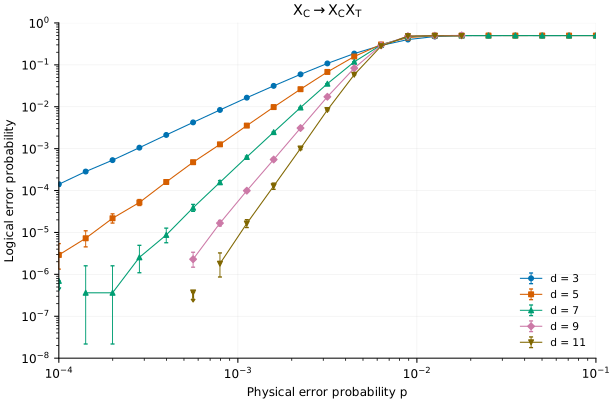
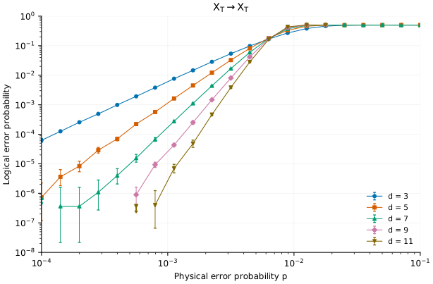
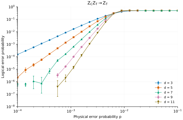
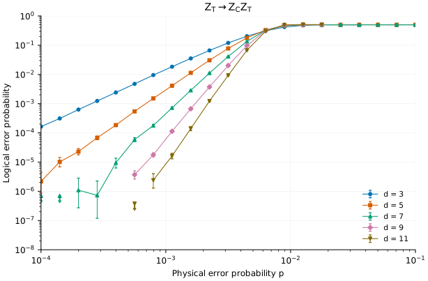
The plots show simulation results for four independent logical observables of the open-port CNOT, labeled by their correlation surfaces.

Logical error probability for X control to X control times X target.

Logical error probability for X target to X target.

Logical error probability for Z control times Z target to Z target.

Logical error probability for Z target to Z control times Z target.

Continue with Logical T Gate to add resource retries and measurement-dependent basis selection.